Maximum likelihood estimators

STA602 at Duke University

Background: likelihoods

Example: normal likelihood

Let \(X\) be the resting heart rate (RHR) in beats per minute of a student in this class.

Assume RHR is normally distributed with some mean \(\mu\) and standard deviation \(8\).

\[ \textbf{Data-generative model: } X_i \overset{\mathrm{iid}}{\sim} N(\mu, 64) \]

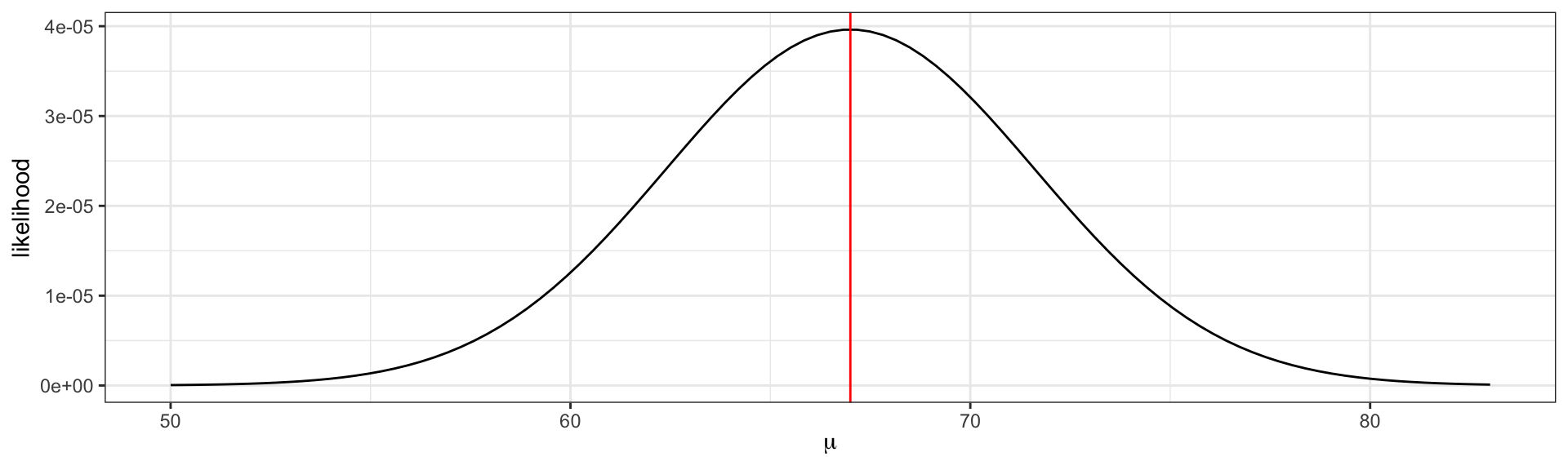
If we observe three student heart rates, {75, 58, 68} then our likelihood \[L(\mu) = f_x(75 |\mu) \cdot f_x(58|\mu) \cdot f_x(68|\mu).\] That is, the joint density function of the observed data, viewed as a function of the parameter.

Important

The likelihood itself is not a density function of the unknown parameter(s). The integral with respect to the parameter does not need to equal 1.

Definition

The likelihood function is the joint density (or mass function) of the data viewed as a function of the unknown parameter(s).

Visualizing the likelihood

\[L(\mu) = f_x(75 |\mu) \cdot f_x(58|\mu) \cdot f_x(68|\mu).\] The maximum likelihood estimate \(\hat{\mu} = \frac{75 + 58 + 68}{3} = 67\).

The maximum likelihood estimate is the parameter value that maximizes the likelihood function.

data

x = c(75, 58, 68)

likelihood function

L = function(mu, x) {
  stopifnot(is.numeric(x))
  n = length(x)
  likelihood = 1
  for(i in 1:n){
    likelihood = likelihood * dnorm(x[i], mean = mu, sd = 8)
  }
  return(likelihood)
}

plot

plot code

ggplot() +
  xlim(c(50, 83)) +
  geom_function(fun = L, args = list(x = x)) +
  theme_bw() +
  labs(x = expression(mu), y = "likelihood") + 
  geom_vline(xintercept = 67, color = 'red')

The log-likelihood

Notice how small the y-axis is on the previous slide. What happens to the scale of the likelihood as we add additional data points?

\[ L(\mu) = \prod_{i = 1}^{n} f_x(x_i |\mu) \]

. . .

Since densities often evaluate between 0 and 1, multiplying many together (as we usually do in likelihoods) can quickly result in floating point underflow. That is, numbers smaller than the computer can actually represent in memory.

• Note: sometimes densities evaluate to greater than 1 (e.g. dnorm(0, 0, 0.001)) and multiplying several together can result in overflow.

. . .

log to the rescue!

• log is a monotonic function, i.e. \(x > y\) implies \(\log(x) > \log(y)\), because of this the maximum of \(f\) is the same as the maximum of \(\log f\).

• additionally, log turns products into sums

in practice, we always work with the log-likelihood,

\[ \log L(\mu) = \sum_{i = 1}^n \log f_x(x_i | \mu). \]

MLE

Maximum likelihood estimation (MLE)

How did we know to take the average of the values to find the maximum likelihood estimator \(\hat{\mu}\)?

. . .

From calculus, we know that to maximize a univariate function, we need to find where the slope equals zero (technically, to ensure we find some maxima and not a minima we need to also check that the second derivative is negative).

Example: normal likelihood

For the normal likelihood example on the previous slide, we can see visually that the function is concave.

Step 1

To find the maximum, take the derivative

\[ \begin{aligned} \frac{d}{d\mu} \log L(\mu) &= \sum_{i}\frac{d}{d\mu} \log f_x(x_i |\mu)\\ &= \sum_{i}\frac{d}{d\mu} \left[ -\frac{1}{2} \log (2 \pi \sigma^2) - \frac{1}{2\sigma^2} (x_i - \mu)^2 \right]\\ &= \sum_i \frac{1}{\sigma^2} (x_i - \mu) \end{aligned} \]

Step 2

Set the derivative equal to zero and solve,

\[ \begin{aligned} \sum_i \left( x_i - \hat{\mu} \right) &= 0\\ n \hat{\mu} &= \sum_i x_i\\ \hat{\mu} &= \bar{x} \end{aligned} \]

Exercise 1: binomial MLE

Let \(Y_1, Y_2, \ldots, Y_n \sim \text{iid } \text{binary}(\theta)\). Here \(\theta\) is the probability of a success, i.e. \(prob(Y_i = 1)\).

• Note: a “binary” distribution is equivalent to a “Bernoulli” distribution. Your book calls it “binary”, so we will as well for consistency.

1. Write down the likelihood, \(p(y_1, \ldots, y_n | \theta)\).

2. Write down the log-likelihood.

3. Compute \(\hat{\theta}_{MLE} = \text{argmax}_{\theta}~ \log p(y_1, \ldots, y_n | \theta)\)

Solution 1

solution 1a

The likelihood

\[ \begin{aligned} p(y_1, \ldots, y_n | \theta) &= \prod_{i=1}^n p(y_i | \theta)\\ &= \theta^{y_i}(1-\theta)^{1-y_i}\\ &= \theta^{\sum {y_i}}(1-\theta)^{n - \sum y_i} \end{aligned} \]

solution 1b

The log-likelihood

\[ \log \left(\theta^{\sum {y_i}}(1-\theta)^{n - \sum y_i} \right) = n \bar{y} \log \theta + n(1-\bar{y}) \log(1 - \theta) \]

where \(\bar{y} = \frac{1}{n} \sum_{i=1}^n y_i\).

solution 1c

Take the derivative \[ \begin{aligned} \frac{d}{d\theta} \log p(y_1, \ldots, y_n | \theta) &= \frac{n\bar{y}}{\theta} - \frac{n - n\bar{y}}{1- \theta} \end{aligned} \]

and set equal to 0. After simplifying,

\[ \hat{\theta}_{MLE} = \bar{y} \]

Exercise 2

Zero-inflated models allow for frequent zero-valued observations. You observe 100 people at the beach fishing. Click “View data” to see the number of fish each individual catches (reported as fishing_count) below.

fishing_count = c(0, 0, 0, 3, 0, 3, 5, 0, 8, 1,
                  0, 0, 0, 0, 3, 4, 0, 4, 8, 0,
                  0, 0, 4, 0, 0, 6, 4, 0, 4, 0,
                  0, 0, 0, 0, 4, 8, 4, 0, 0, 0,
                  7, 3, 0, 2, 0, 0, 7, 7, 5, 0,
                  0, 0, 7, 6, 0, 3, 0, 0, 0, 5,
                  4, 1, 0, 0, 0, 0, 0, 0, 0, 8,
                  0, 5, 0, 3, 0, 0, 3, 0, 0, 2,
                  0, 5, 0, 7, 7, 0, 1, 0, 2, 7,
                  0, 2, 4, 0, 0, 1, 5, 0, 0, 0)

The data can be described as being generated from a zero-inflated mixture model. Let be the number of fish an individual catches at the beach,

\[ \begin{aligned} p(Y_i = 0) &= p +(1 - p)e^{-\lambda}\\ p(Y_i = y_i) &= \frac{(1-p) \lambda ^ {y_i} e^{-\lambda}}{y_i!}, ~y_i = 1, 2, 3, \ldots \end{aligned} \]

Assume observations \(Y_1, \ldots, Y_{100}\) are independent.

1. Write down the log-likelihood and visualize the log-likelihood as a function of \(p\) while fixing \(\lambda = 5\). Repeat for \(\lambda = 4\) (on the same plot).

2. Based on your plot, which value of \(\lambda\) is more likely? Assuming these \(\lambda\) are sufficiently close to the true \(\lambda\), what is (approximately) the MLE of \(p\) based on your plot?

3. Can you find a closed form solution for \(\hat{\lambda}_{MLE}, \hat{p}_{MLE}\)? Why or why not?

Solution 2

a (log-likelihood)

\[ \log \left(p(Y_i = 0)^{57}\prod_{i = 1}^{43} p(Y_i = y_i) \right) = \\ 57 \log p(Y_i = 0) + \sum_{i = 1}^{43} \log p(Y_i = y_i) \]

where

\[ \begin{aligned} p(Y_i = 0) &= p + (1-p) e^{-\lambda}\\ p(Y_i = y_i) &= \frac{(1 - p)\lambda^{y_i}e^{-\lambda}}{y_i!}, \ \ y_i = 1, 2, 3, \ldots \end{aligned} \]

a (code)

sum(fishing_count == 0)
fishing_subset = fishing_count[fishing_count != 0 ]
length(fishing_subset) # sanity check

probYzero = function(p, lambda) {
  prob1 = log(p + ((1 - p) * exp(-lambda)))
  return(57 * prob1)
}

likelihood = function(p, lambda) {
  total = 0
  for (i in seq_along(fishing_subset)) {
    total = total +
      (log(1 - p) + (fishing_subset[i] * log(lambda)) - lambda) -
      log(factorial(fishing_subset[i]))
  }
  return(probYzero(p, lambda) + total)
}
ggplot() +
  xlim(c(0.0, 1)) +
  geom_function(fun = likelihood, args = list(lambda = 8)) +
  geom_function(fun = likelihood,
                args = list(lambda = 4),
                col = "red") +
  theme_bw() +
  labs(x = "p", y = "log-likelihood")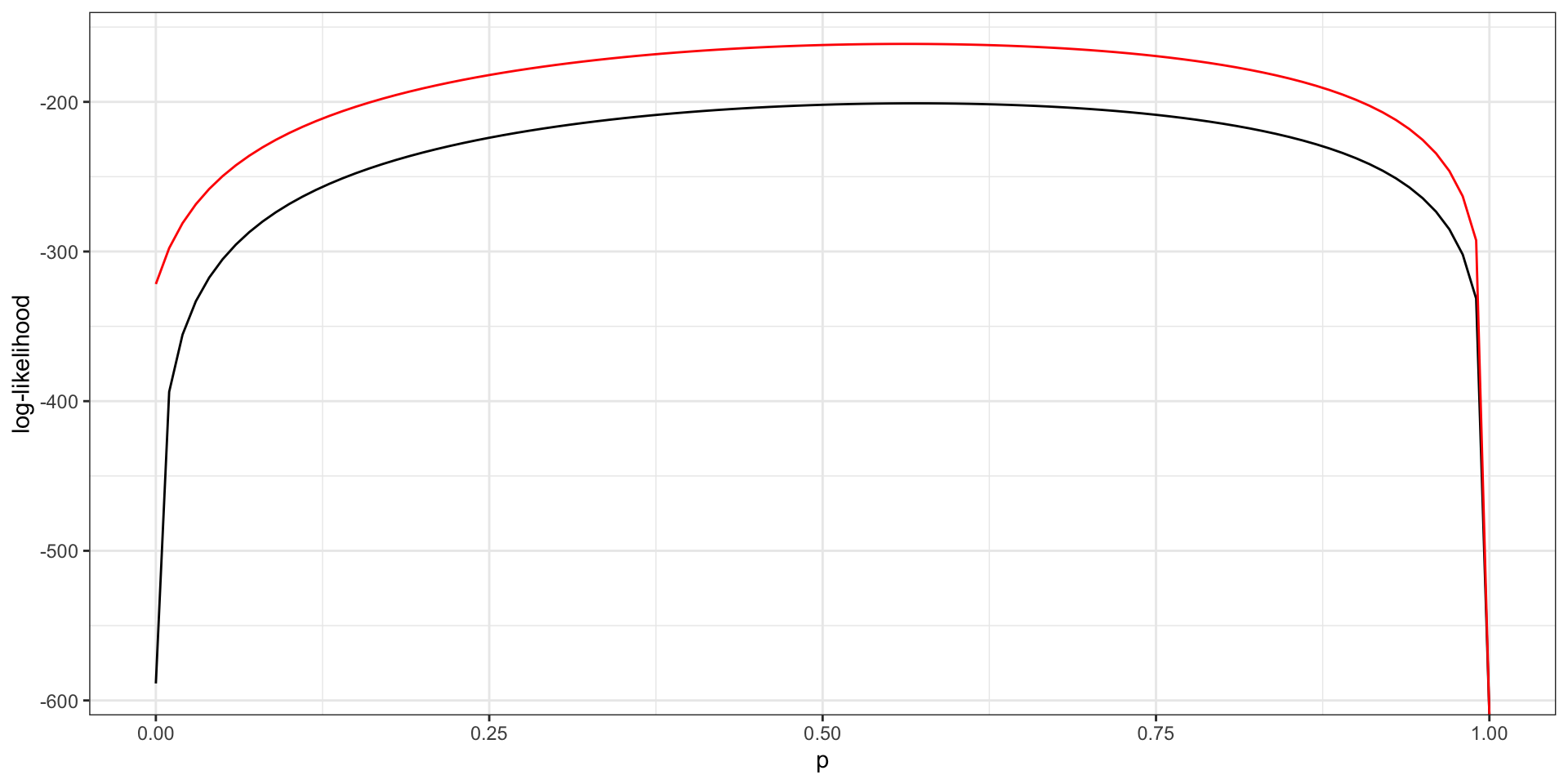

a (plot)

b

• \(\lambda = 4\) is more likely.
• \(\hat{p}_{MLE} \approx 0.5\).

c

Take the gradient and set equal to zero. Two equations and two unknowns, but you cannot isolate \(\hat{\lambda}\) when taking the derivative with respect to \(\lambda\). No closed form solution, need to solve numerically, e.g. with Newton’s method.